Tracing Back to the Origins | The MP Neuron "Logical Calculus of the Ideas Immanent in Nervous Activity" (1943)
Introduction
This article discusses the paper A Logical Calculus of the Ideas Immanent in Nervous Activity [1], published in 1943 by biologist Warren McCulloch and logician Walter Pitts. In Chinese, it translates to The Logical Calculus of Ideas in Nervous Activity. Before reading this article, I suggest reading the introductory piece to better understand the symbolic systems used in the paper. Recently, I’ve been diving into some “classical” papers (often regarded as foundational in modern AI development). However, finding the content challenging and lacking detailed analysis, I managed to piece together a basic understanding during my spare time. I hope this “back-to-basics” article can aid learners with similar interests who may not know where to start. 😊
This article is around 5000 words, estimated reading time is 20 minutes.
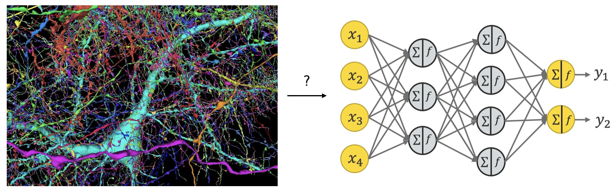
If we were attending a general introduction to artificial intelligence, the instructor would likely start with artificial neural networks (ANNs) and introduce the basic structure of input layers, hidden layers, and output layers, as shown on the right side of Figure 1. The weighted sum of neuron outputs, passed through an activation function
Introduction
The article begins with several key points in the Introduction (not analyzed here word-for-word, but you can search online for a PDF copy; the content, being rather old, can be difficult to read, especially for non-biology majors, like me):
- Neural activity has an “all-or-none” nature (neural activity is either present or absent, akin to 0 or 1, true or false).
- To trigger a pulse in the next neuron, a certain number of synapses must activate within a specific time frame (each neuron has a threshold independent of its position and previous activity).
- The only significant delay in the nervous system is synaptic conduction delay (axon delay can be ignored).
- Inhibitory synapses prevent neuron activation at certain times (explains the refractory period of neurons using inhibitory synapses).
- The structure of neural networks does not change over time (long-term phenomena like learning and extinction are broadly equivalent to the original network).
Based on these assumptions, we define some symbols. If this part seems hard to understand, consider reading the preliminary article.
Definitions
We first define a functor
where
Now, we define the structure of a neural network
where
Oppositely, consider a predicate
To interpret these definitions, narrow realizability is a stringent condition requiring a specific neural network structure to directly achieve a particular state described by the predicate through specific neuron arrangements and input substitutions. Conversely, extended realizability is a more lenient condition, allowing multiple applications of functor
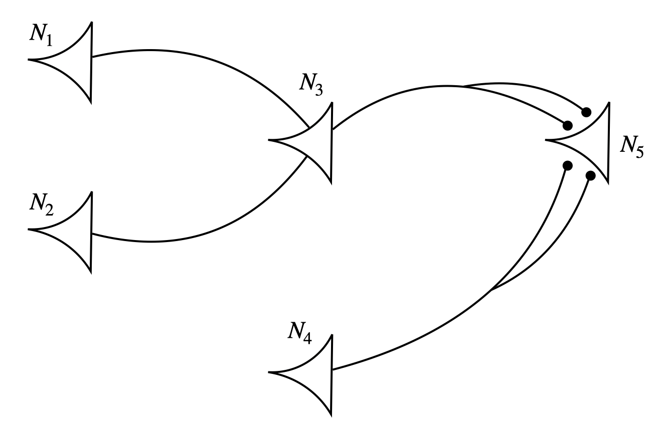
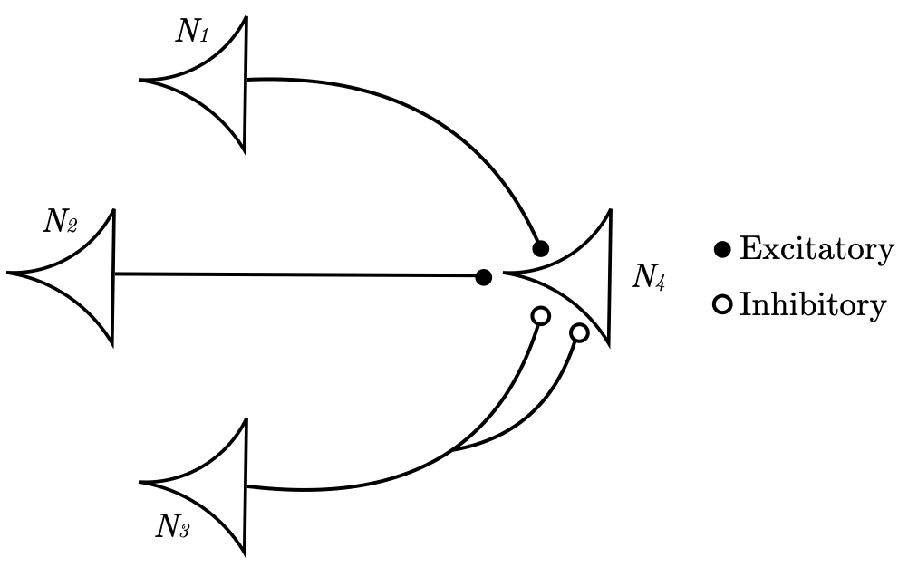
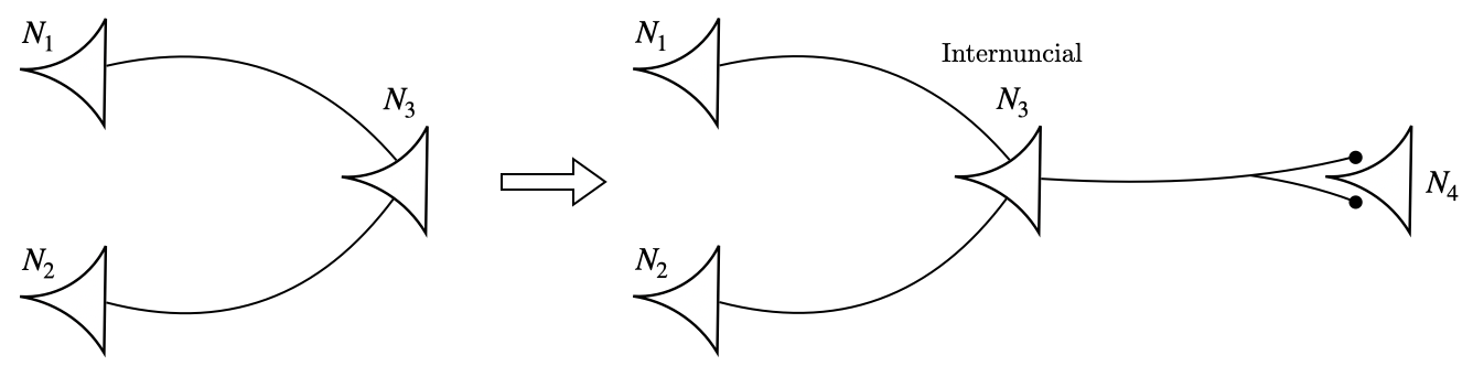
Let’s consider a simple example (Figure 3). First, take the expression
Finally, we arrive at the last definition! The paper defines Temporal Propositional Expressions (TPE) using recursive rules.
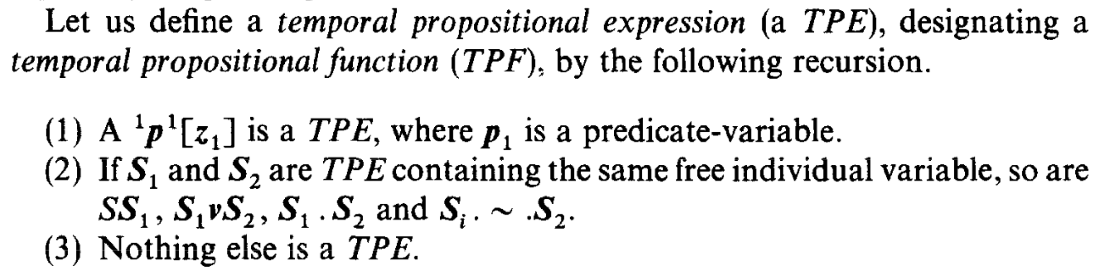
First,
Review
We defined functor
- Find an effective method to obtain a computable set of
that forms the solution for any given network (calculate the behavior of any network). - Describe a set of realizable solutions.
In simple terms, the problems are (1) to calculate any network’s behavior and (2) to determine networks that manifest as specific states.
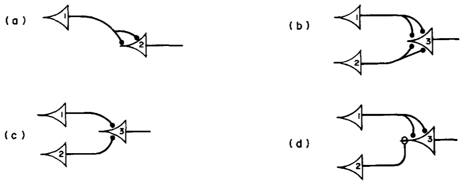
Theorems and Simple Proofs
Note 1: A 0th-order neural network refers to a network without circular structures. The latter half of the paper provides detailed explanations for nets with circles, which are not covered here.
Theorem 1. Every 0th-order net can be solved in terms of Temporal Propositional Expressions (TPEs).
Let
where
Assuming a threshold of two, it’s clear that
Theorem 2. Every TPE is realizable by a 0th-order network in the extended sense.
Note 2: The term “realizable in the extended sense” is abbreviated as “realizable” in the proof.
The second theorem states that for any neuron state description, there exists a 0th-order network that realizes it in the extended sense. The proof of Theorem 2 provides a recursive method for constructing a 0th-order network that realizes a TPE.
Since functor
Consider a proposition
Thus, if
Based on the previous conclusions,
Theorem 3. Let there be a complex sentence
Though complex at first glance, Theorem 3 provides the criterion for determining whether an expression is a TPE. In other words, it gives a method for determining if an expression is a TPE. There are three equivalent methods:
- The composite sentence is false when all its basic sentences are false.
- The last line of the truth table contains “false.”
- There is no term in its Hilbert Disjunctive Normal Form (HDNF) composed solely of negated terms.
Let’s examine a few examples for each condition:
- For the composite sentence
, where and are basic propositions. When both and are false, is also false, i.e., . Therefore, satisfies the first condition and is a TPE. - For the composite sentence
, the truth table is as follows: 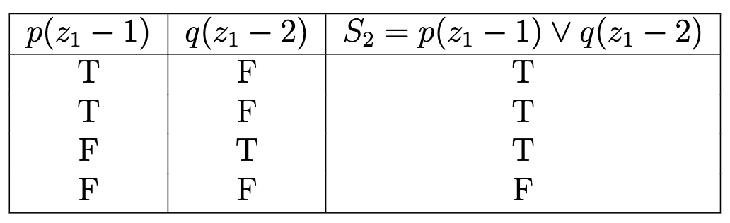
As shown, when bothand are false, is also false. Hence, satisfies the second condition. - For the composite sentence
, converting it to HDNF gives . In HDNF, the only term consists solely of negated terms. Therefore, does not meet the third condition and is not a TPE.
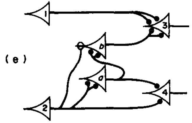
Now, let’s apply these theorems to implement a neural network. Consider a scenario: when an ice cube touches and then leaves our skin for a moment, we feel heat before coolness; but if it stays longer, we only feel a chill. To model this situation, let
Since these sentences are already in Hilbert Disjunctive Normal Form (HDNF), Theorem 3 indicates that both
Finally, the paper mentions that different inhibition phenomena are broadly equivalent (2) extinction and learning are equivalent to absolute inhibition. If these two conclusions are proven, it indicates that the current structure simulates actual neural networks, allowing us to compute any network’s behavior and determine networks manifesting specific states. This part is briefly discussed in the original paper, so we will not explain the details it here.
Summary
The McCulloch-Pitts neuron model simplifies neuron behavior into logical operations, executing basic logic through “all-or-none” responses. Its significance lies in formalizing the behavior of neural systems, demonstrating the Turing completeness of neural networks, capable of simulating any state. This groundbreaking theory laid a solid foundation for the Perceptron and propelled the development of artificial neural networks (ANNs). (Spoiler alert: the next topic will be Perceptron or theories related to emergence, expected within three days 🤞).
End
References
[1] McCulloch, W. S., & Pitts, W. (1943). A logical calculus of the ideas immanent in nervous activity. The Bulletin of Mathematical Biophysics, 5(4), 115–133. https://doi.org/10.1007/bf02478259
[2] Marshall, M. (2021, June 7). Google has mapped a piece of the human brain in the most detail ever. New Scientist; New Scientist. https://www.newscientist.com/article/2279937-google-has-mapped-a-piece-of-human-brain-in-the-most-detail-ever/
[3] A Friendly Introduction to [Deep] Neural Networks | KNIME. (2021). KNIME. https://www.knime.com/blog/a-friendly-introduction-to-deep-neural-networks