Tracing Back to the Origins | "Perceptron" The Intelligent Machine (1957)

Preface
Continuing from the last article in our “Tracing the Roots” series, we’ll delve into a pioneering work in the field of artificial intelligence that followed the MP neuron model: the Perceptron. This article will give a detailed analysis of the 1957 paper, The Perceptron: A Probabilistic Model for Information Storage and Organization in the Brain, by Frank Rosenblatt, a psychologist and neuroscientist at Cornell University.

Introduction
At the beginning of the article, the author presents three fundamental questions for understanding cognition, generalization, memory, and thought:

1. How do biological systems perceive or detect information from the physical world?
2. In what form is information stored in memory?
3. How does stored information influence recognition and behavior?

The first question has largely been addressed in sensory physiology. For the second and third questions, the author discusses two perspectives:

• The Coded Memory Hypothesis suggests that information is stored in an encoded form, like a wiring diagram, that can directly translate sensory input into memory. Recognizing external stimuli involves matching the current sensory pattern with stored content and mapping it to a corresponding response.
• The Empiricist Memory Hypothesis proposes that information storage does not involve specific encoding but occurs through forming new connections in the nervous system. Since the information is stored as neural connections, new stimuli use these established pathways, triggering an appropriate response without needing a separate recognition process.

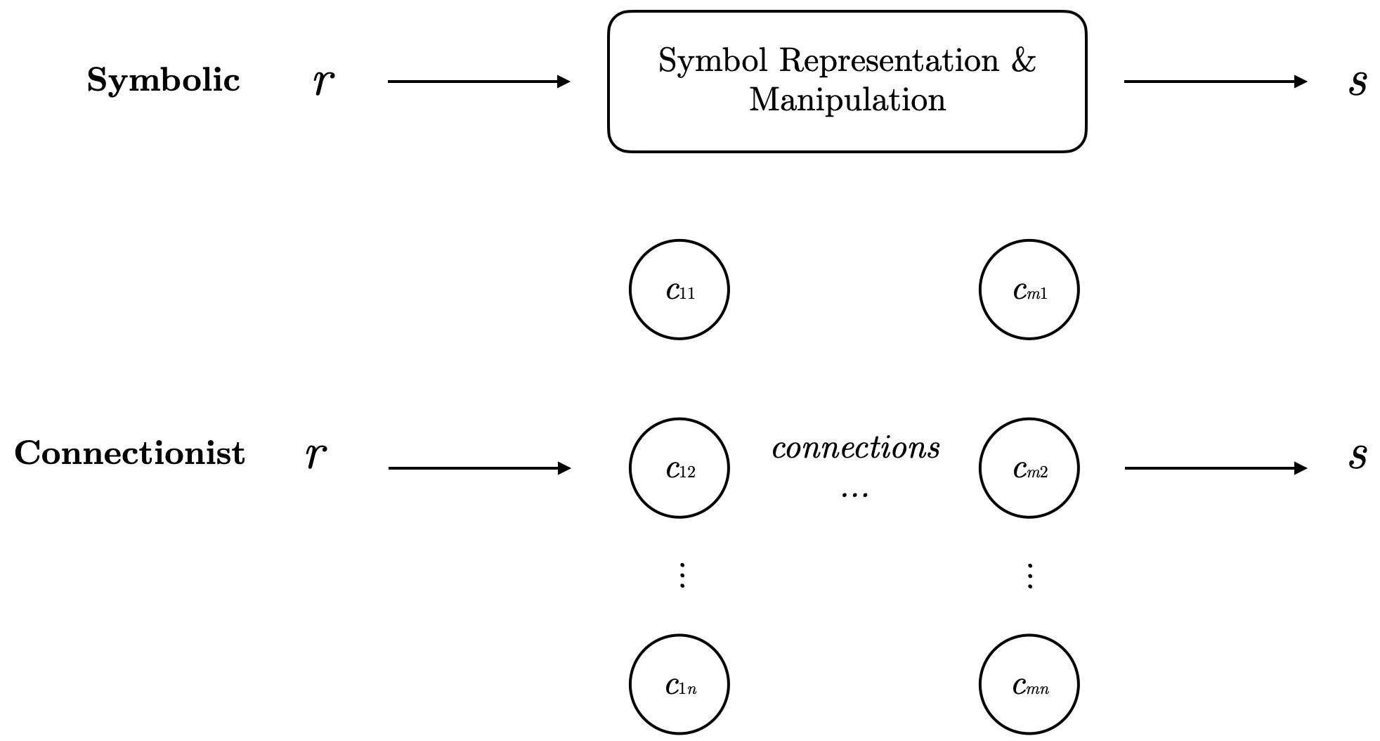
These two hypotheses can actually be mapped to two major schools of artificial intelligence: Connectionism and Symbolism. Symbolism assumes cognitive processes are achieved through clear symbol manipulation and sequential application of rules. In contrast, Connectionism models cognition by simulating neural networks, relying on distributed representations and statistical methods.

In the previous article, we discussed MP neurons, which are based on Boolean logic and binary operations. In the Perceptron paper, the author critiques symbolic methods. These theorists focus on implementing functions like perception and memory using deterministic physical systems rather than studying how the brain actually performs them. Many of the proposed models fail in important ways: they lack consistency across different situations (equivalence), they don’t use neural resources efficiently (neuroeconomy), they impose strict requirements on connections (excessive specificity), and the variables in the models lack biological evidence. Supporters of these physical systems argue that biological intelligence can be replicated by improving existing principles. However, the author believes these limitations show that models not based on biological systems can never explain biological intelligence, as the difference in principles is clear.

Conversely, studies that focus on biological systems often lack precision and rigor, making it difficult to assess whether the described systems can actually work in real neural networks. The lack of an analytical language as effective as Boolean algebra is another obstacle.

To address these issues, the author first introduces several key assumptions:

1. The construction of the neural system’s initial network is largely random, with minimal genetic restrictions.
2. Neural connections exhibit some plasticity. After a period of neural activity, the probability of stimulating one group of cells and triggering a response in another group changes due to long-term changes in neurons.
3. Similar stimuli tend to form pathways to the same responsive cells, and vice versa.
4. Positive and negative reinforcement promotes or inhibits the formation of connections.
5. Similarity isn’t an inherent attribute of specific stimuli but depends on the physical organization of the perceptual system.

These assumptions will serve as essential foundations for the model. Unlike previous work, the Perceptron uses a probabilistic model rather than Boolean operations.

The Basic Structure of the Perceptron
The following is a simple diagram of the perceptron’s structure:

Fig. 2: A Simple Diagram of the Perceptron Structure.

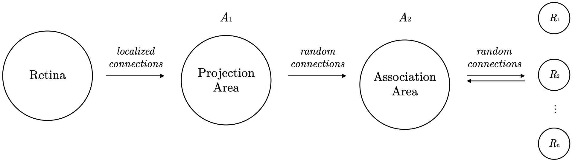
The model is organized into four parts:

1. Sensory Input Layer: The perceptron’s input comes from sensory receptors, like retinal points, labeled S-points, that respond in an “all-or-none” manner to stimuli. Note: “All-or-none” means that if the stimulus weight exceeds the neuron’s threshold , the neuron activates; if not, it remains inactive.
2. Projection Area: The S-points send signals to a projection area (a group of associated cells labeled , with neurons referred to as A units). The activation of A units follows the same “all-or-none” rule. Notice the localized connections here: A units’ source points tend to cluster around each A unit’s central retinal point. The number of origin points decreases exponentially with distance from the central point. This distribution is vital in contour detection, making it a bio-inspired design. Sometimes, the projection area is omitted during modeling.
3. Association Area: Each A unit in the association area receives signals from multiple source points, and connections between the two regions are random.
4. Response Layer: Outputs from the association area go to response cells (labeled R units). While the perceptron uses feedforward connections until the association area, feedback is provided in the response layer. The author suggests two almost equivalent feedback mechanisms:
   • (a) Excitatory feedback to the source cell set of an R unit.
   • (b) Inhibitory feedback to the complement of the source set of an R unit.

In this system, based on feedback, the neurons’ responses are mutually exclusive. If one response unit is activated, it inhibits the set of cells connected to another response unit , preventing from responding. As reinforcement and inhibition continue, the system gradually adapts to stimuli of different categories—a process we describe as learning ability.

For simplification in later analysis, only Sensory Input - Association Area - Response Layer are kept. The A unit represents neurons in the association area, and the R unit represents neurons in the response layer. To simplify further, the author distinguishes between two response phases:

Fig. 3: Response Phases to Stimuli.

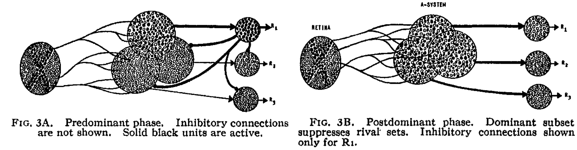
• Predominant Phase: A units in the system respond to stimuli, but R units remain inactive. This phase is temporary and transitions to the Postdominant phase.
• Postdominant Phase: One R unit becomes active, dominating by suppressing other activities in its source set.

In the predominant phase, responses are random. However, as stimulus-response connections are reinforced, the system learns to respond to specific stimuli. Below, we discuss the characteristics of each neuron in the macrostructure.

Modeling Neuron Characteristics

To address assumption two (neural plasticity) and to enable the Perceptron’s dynamic learning process, we introduce a model for neuron characteristics, which will serve as the foundation for subsequent simulations.

Assume that each A unit’s output impulse can be represented by a value , which could reflect amplitude, frequency, delay, or transmission probability. A higher value indicates that all output impulses of an A unit are more effective or more likely to reach the response layer. Each A unit’s value is assumed to be relatively stable (determined by the cell membrane and metabolic state of the cell), but it is not constant. We generally assume that activity increases the cell’s value, while inactivity decreases it.

An interesting model is one where cells compete for metabolic materials, with more active cells drawing from inactive ones. In such a system, without activity, all cells’ states would stabilize, resulting in a net value balance across the system. The author introduces three systems () with different rules for changes in neuron values :

Fig. 4: Comparison of Three System Logic Characteristics.

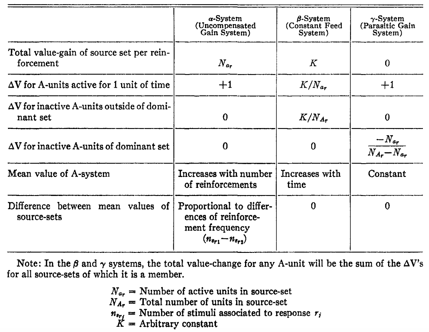
• System (Uncompensated Gain System): Each time an A unit receives a stimulus, it gets a fixed gain, accumulating over time without decreasing. This cumulative gain mechanism is suited for tasks with long-term accumulation effects.
• System (Constant Feed System): Each source set gains at a constant rate, with distribution proportional to the activity in the set. Non-dominant set cells also receive gains, ensuring all units have the chance to activate and strengthen over time. This balanced mechanism supports ongoing learning and stable gain distribution.
• System (Parasitic Gain System): Active cells gain values at the expense of inactive ones, keeping the total source set value constant. This competitive mechanism is suitable for tasks focused on resource optimization.

The next section builds learning curves and performs a sensitivity analysis on the model.

Model Analysis of the Predominant Phase

To compare learning curves, we define two key metrics:

• : The expected proportion of A units activated by a given stimulus. This is calculated by summing over all possible excitatory () and inhibitory () inputs under the condition that the sum of excitation minus inhibition reaches or exceeds the threshold (). represents the joint probability of excitatory and inhibitory components; is the total excitatory connections per A unit, is the total inhibitory connections, and is the proportion of S-points activated before each A unit.
  

• : The conditional probability that an A unit responding to a stimulus will also respond to a different stimulus :
  
  Here, and are the counts of excitatory and inhibitory source points “lost” when is replaced by , while and are the counts of points “gained” when is replaced by . The joint probability is as follows:
  
  Here, is the proportion of S-points lit by but not , and is the proportion of S-points remaining from that are included in . Let’s examine how and change with parameter variations.

Sensitivity Analysis of

Using the formula and rules discussed, we can plot graphs (code available in repository):

Fig. 5: Variation of with the proportion of retina area illuminated (R).

Conclusions:

1. Increasing the threshold or increasing inhibitory connections reduces .
2. When excitatory and inhibitory inputs are roughly balanced, the curve flattens with changes in .
3. Systems with similar amounts of excitatory and inhibitory input converge faster. For optimal stability, a balance of excitatory and inhibitory input is desirable.

Sensitivity Analysis of

Fig. 6: Variation of with .

1. As increases, decreases faster than .
2. Like , decreases as the proportion of inhibitory connections increases.

Additionally, the author explored how changes with stimulus overlap , as shown below:

Fig. 7: Variation of with . Solid line represents , dashed line represents , with and .

1. Even when stimuli are entirely non-overlapping, remains above zero, showing that the system can still respond to completely different stimuli.
2. As overlap increases, approaches 1, indicating strong consistency in system response.
3. Higher threshold values result in lower values compared to lower thresholds.

Analyzing and provides a theoretical basis for quantitative analysis and parameter tuning. Summing up the insights gained:

• Symbolism vs. Connectionism
• Transition from formal logic to probabilistic models in neural networks
• The foundational structure and functioning of the perceptron
• Neuron characteristic modeling with three systems
• Learning curve development and sensitivity analysis
• Convergence based on different criteria

The second half of the original paper focuses on the perceptron’s spontaneous organization, memory and learning capabilities, and the model’s performance in varied environments. We won’t cover this section here, as it primarily involves small-scale experiments and fine-tuning rather than the foundational contributions of the first half.

A major limitation of the Perceptron is that it can only solve linearly separable tasks, struggling with non-linear ones. This led to the development of the Multilayer Perceptron with non-linear activation functions in hidden layers, allowing for non-linear classification. However, challenges remain, especially with training. Next time, we’ll explore the 1986 paper by Hinton, Rumelhart, and Williams, Learning Representations by Back-Propagating Errors, which made training deep neural networks feasible.

(P.S. Thanks for reading! A like would mean the world 😊)