Tracing Back to the Origins | Back-propagation "Learning representations by back-propagating errors"（1986)

Preface

Following the previous article in the “Tracing the Origins” series, where we explored the MP neuron, we now dive into a groundbreaking advancement in the field of AI, the Perceptron, introduced in the 1957 paper by Frank Rosenblatt. This article will deeply analyze the 1986 paper Learning Representations by Back-Propagating Errors [1] by Rumelhart, Hinton, and others, which introduces the well-known backpropagation learning method. This method aims to minimize the discrepancy between a neural network’s actual and desired outputs by adjusting connection weights within the network, thus enabling it to learn and optimize internal representations for complex tasks. This paper not only laid the theoretical foundation of modern deep learning but also sparked extensive exploration into neural networks’ practical applications. At the end of this paper, the authors presented some fascinating insights from today’s perspective, worth exploring further.

Introduction

Scientists have made numerous attempts to design self-organizing neural networks. Their goal was to find an effective method for learning and self-adjusting connections within the network to automatically find the right connections and states for specific tasks. If inputs and outputs are directly connected, finding a way to learn is relatively straightforward: one only needs to repeatedly adjust the strength of the connections so that the output gradually approximates the target result. However, networks that directly connect outputs and inputs can only address linearly separable problems. For example, if we have a basket of apples and watermelons that differ in size and dimension, we could use a straight line to separate apples and watermelons on a size-weight chart. In such problems, a line or hyperplane can fully separate data points in a 2D or multidimensional space. However, many real-world data features do not exhibit clear distinctions, such as movie review sentiment (positive or negative?) or stock market predictions (rise or fall?), which cannot be split by a simple linear boundary.

To tackle these linearly inseparable problems, the concept of hidden layers was proposed. The state of hidden layers is not directly given but must be learned to determine which stimuli activate neurons, layer by layer, to ensure the network produces the correct output. In the Perceptron model, although the association area sits between inputs and outputs, its connections are fixed and do not adapt through learning. In this paper, the authors found a simple yet powerful method—the backpropagation algorithm—capable of automatically adjusting hidden units to build internal representations suited to task requirements. We will first explain the core of backpropagation, introduce specific examples from the authors, and discuss algorithm improvements and intriguing questions.

Backpropagation

This section covers the backpropagation calculation process, with the specific weight update rules explained in the next section.

Consider a layered network consisting of input units, an arbitrary number of hidden layers, and output units. Each layer’s units set their states, beginning with the input units and working up to the output units. Figure 1 provides a simplified illustration of neuron connections and calculations in the paper:

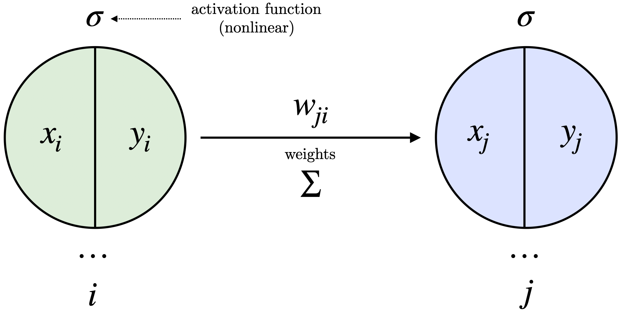
Figure 1: Weighted connections, activation functions, and outputs between adjacent layers.

The total input to neuron is a linear function of the outputs from connected units and the weights of those connections :

where and represent the indices of neurons in the preceding and following network layers, referred to simply as “neuron ” and “neuron .” Additionally, a constant offset, known as a bias, may be added to the neuron’s total input. With the bias, the input can be written as:

The real-valued output of the neuron is a nonlinear function of its total input :

The Sigmoid function is a commonly used activation function, with all output values between , and it has a straightforward derivative . The structure of artificial neurons is analogous to biological neurons, as shown in Figure 2.

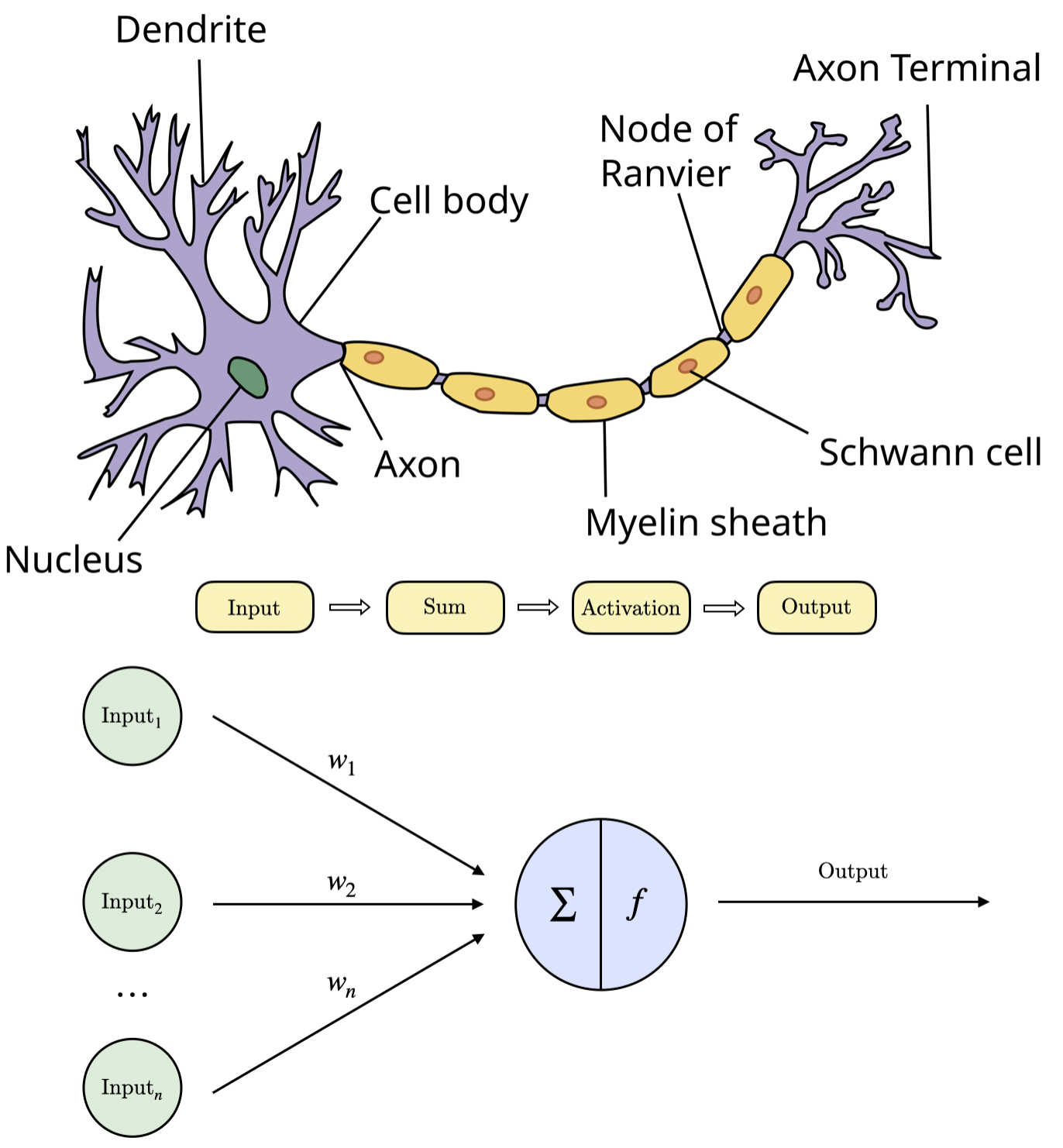
Figure 2: Comparison of biological and artificial neurons—input, summation, activation, and output.

Our ultimate goal is to ensure that for each input vector, the network generates an output vector that matches or closely approximates the desired output vector. The total error of the network can be computed by comparing the actual output vector and the desired output vector:

where is the sample index, is the output unit index, is the actual output unit state, and is its desired state.

For a given data sample, the partial derivative of the error with respect to each weight is calculated through two passes. The state of each layer’s units is determined by the output received from the previous layer’s units. Backpropagation, however, is more complex. Weight derivatives will propagate from the output layer down to the lower layers, using to adjust the weights. Figure 3 illustrates the backpropagation calculation flow.

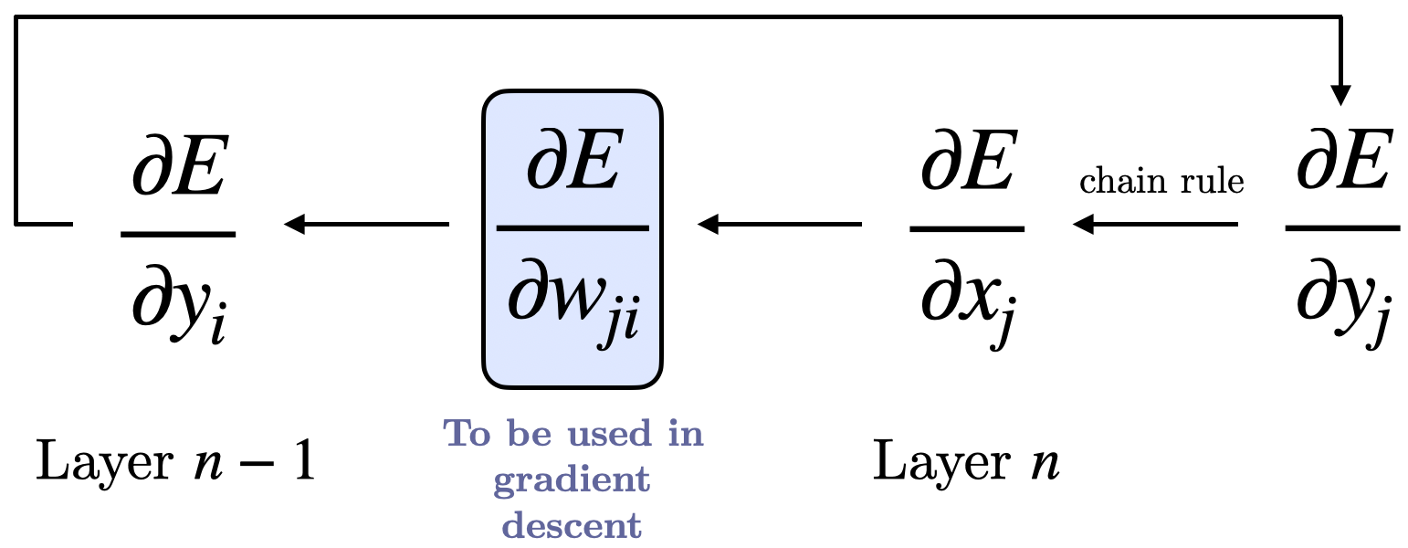
Figure 3: Partial derivative calculation flow.

Consider a specific sample , calculating for the output unit:

Applying the chain rule yields :

Differentiating equation (2) yields , and substituting:

This shows how the total input to the output unit affects error . Since the total input is merely a linear function of lower-unit states and connection weights, we can calculate how weight changes impact the error. For weight connecting unit to unit :

Thus, we have completed one layer’s propagation. To obtain for each layer in the network, continue solving for for preceding layers.

For any output unit , derives from ’s influence on :

Equation (7) provides the method to calculate for any unit in the penultimate layer, once the values for the final layer are given. Repeat this process to compute weight-error derivatives, using to update the gradient.

Using the Gradient to Update Weights

A common method to reduce total error and match outputs with expectations is gradient descent to minimize . Gradient descent is like descending a mountain—finding the weight setup that minimizes error requires constantly scanning for the steepest slope (computing the gradient) and taking appropriate steps (learning rate) until the current weights reach the lowest point.

The simplest form of gradient descent involves modifying the weights by an amount proportional to :

where is the learning rate. This method’s convergence speed is slower than methods that use second-order derivatives but is simpler and can be implemented easily on parallel hardware with local calculations. However, this method encounters a problem: if the learning rate is too large, weights may oscillate near the minimum without ever converging, as shown in Figure 4.

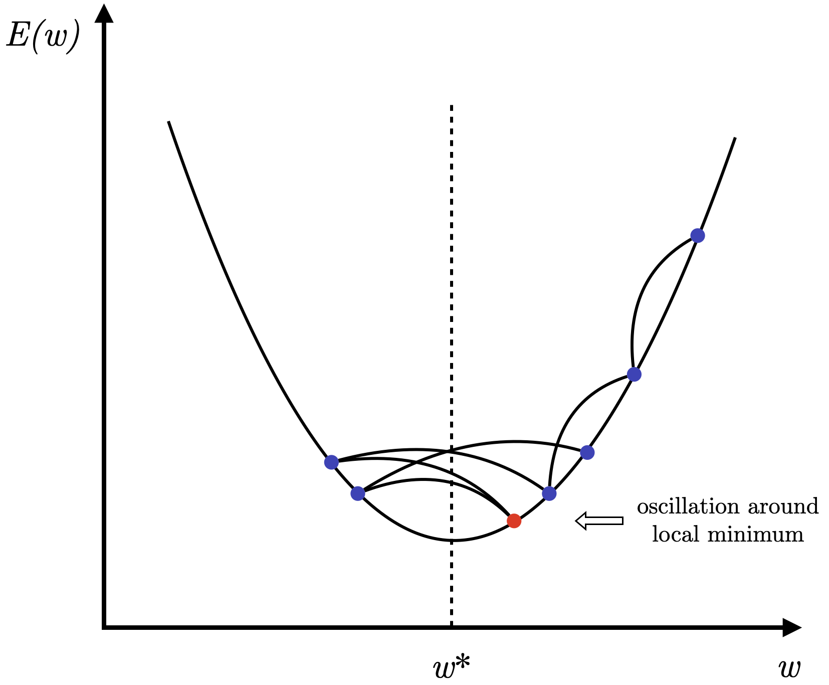
Figure 4: Oscillations around a local minimum.

On the other hand, if the learning rate is too small, convergence will be very slow and equally impractical. The paper suggests a simple acceleration method—momentum—that can significantly improve convergence speed without sacrificing algorithm simplicity:

Here, increments by 1 with each pass through the entire input-output dataset, and is an exponential decay factor between 0 and 1, determining the relative contributions of current and past gradients to weight changes. The momentum method adds “inertia” to gradient descent. Just as in physical movement, inertia keeps an object moving in the same direction without external forces. In gradient descent, this method combines the current gradient with a portion of the previous gradient to update weights, speeding convergence in flatter regions and helping parameters quickly approach the optimal solution.

One last point to mention is the starting values for weights. If all neurons in the network are initialized with the same weights, they will receive identical gradients during training and update identically, limiting the network’s learning ability. To break this symmetry problem, weights are initialized randomly.

The next section will cover some interesting tasks proposed by the authors.

Several Interesting Cases

1. Symmetry Detection Network

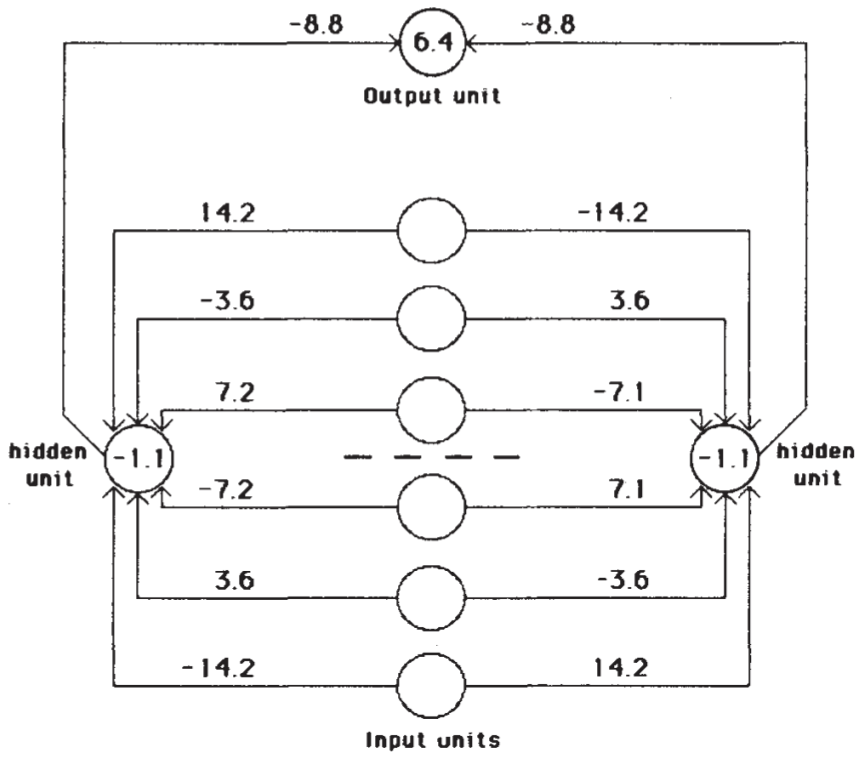
Figure 5: A network that learns to recognize mirror symmetry.

The goal of this task is for the neural network to recognize symmetrical patterns like in a binary vector of length 6. The network consists of six input units, two hidden units, and a single output unit. The model was trained using initial weights randomly distributed between -0.3 and 0.3 and completed 1,425 passes, each time going through all possible input vectors. The learning rate was set to , and the momentum factor was .

Here’s an analysis of what the network learned in Figure 5. For each hidden unit, the weights are equal in magnitude and opposite in sign. The hidden units have a negative bias (-1.1): when the net input to the hidden units is 0, the hidden units remain inactive; the output unit has a positive bias (6.4): when both hidden units are inactive, the output unit activates. The weight ratio for neurons on either side of the midpoint is 1:2:4, so the activation sum sent to the hidden units for each pattern is unique, and only symmetrical patterns completely balance this sum below the midpoint. When the input vector is symmetrical, the opposing weights cancel each other out, resulting in a net input of 0 for each hidden unit. Consequently, the hidden units remain inactive due to their negative bias, while the output unit activates because of its positive bias, detecting the symmetric pattern.

2. Family Tree Network

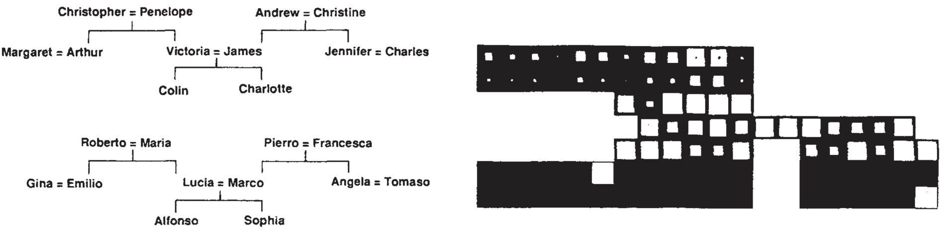
Figure 6: (Left) Two isomorphic family trees; (Right) Activity levels in the family tree network.

Information about the family tree can be represented as triples (person1, relationship, person2), where possible relationships include father, mother, brother, sister, etc. If our network can produce the third element given the first two, it means it has successfully learned these triples.

The training dataset consists of binary vectors of 0s and 1s, with each person and relationship represented by a one-hot encoding. For instance, “Colin” might be represented by a one-hot vector (24 bits), while the “has-aunt” relationship might be (12 bits). The input vector is a concatenation of one-hot encoding vectors for person and relationship, forming a binary vector of length 36 (24 + 12). The family tree network training involved 1,500 passes; the first 20 passes used and , and the remaining used and .

The two groups of white blocks on the right side of Figure 6 show each unit’s activity level. In the first group, one active unit represents Colin; in the second group, one active unit represents the “has-aunt” relationship. Each input group is connected to a hidden layer of six units, with both hidden layers connected to a central layer of 12 units, transitioning to the penultimate layer of six units. This layer’s activity will activate the correct output unit, with each output unit representing a specific person (person 2). The two black dots in the white box mean that (Colin)(has-aunt) has two correct answers—Colin has two aunts.

3. Iterative Network and Equivalent Neural Networks

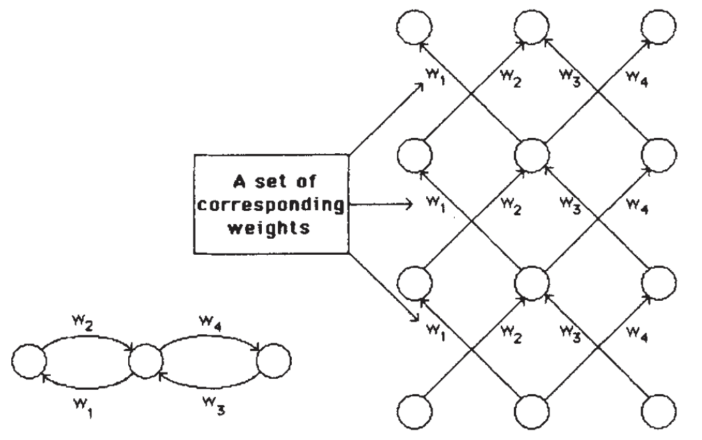
Figure 7: A recurrent neural network and an equivalent neural network.

Figure 7 illustrates a recurrent neural network, where each weight update corresponds to a layer in a layered network. When creating a layered structure equivalent to a recurrent network, two challenges arise:

• Storing Each Unit’s Output State History: In the layered network, intermediate layer outputs are necessary during backpropagation. Therefore, in an iterative network, each unit’s output state history needs to be stored for use in backpropagation.
• Ensuring Weight Consistency: To maintain equivalence between the layered and iterative networks, weights between different layers must have the same value. This can be achieved by averaging each corresponding weight’s value and adjusting each weight in proportion to the average gradient:
  
  With these two modifications, the learning process described above can be applied directly to iterative networks.

Conclusion

The models and cases are now covered; this straightforward algorithm enables neural networks to learn complex, nonlinear patterns and has driven the development of many modern deep learning techniques. At the end of the paper, the authors note: the forward-propagation–loss-calculation–backpropagation learning process may not be entirely plausible from a biological perspective, but it performs exceptionally well in practice. Therefore, we must continue searching for algorithms that more accurately reflect biological principles.

However, from today’s perspective, structures like ResNet, Transformer, and many network architectures and optimization algorithms bear little relation to biology or neuroscience. On the other hand, some people question whether deep learning, known for “Money is all you need,” will lead us toward true AGI. Has AI taken the wrong path? Returning to the point made at the end of the backpropagation paper: does achieving intelligence require neuroscientific evidence? Could interdisciplinary work in biology, philosophy, and computer science be the key to solving these issues in the future?

For these big questions, I believe we can consider artificial intelligence and intelligence separately in our research. The term “artificial intelligence” often leads us into the vortex of ethical debates about technology, yet it may also be somewhat misleading. Intelligence involves more than reasoning, computation, and decision-making behaviors; it also ties to complex emotions and consciousness issues. The term “neural network” evokes ideas of intelligence, but we can equally describe it as “an input-hidden-output model based on error calculation and parameter optimization.” On one hand, how to responsibly apply AI might be a more urgent, practical question than “are we on the wrong path.” Besides, whether humanity needs to replicate intelligent conscious entities is still debatable.

Nonetheless, I still believe AI offers an excellent starting point for us to build complex interdisciplinary links, unraveling questions of intelligence and consciousness from a quantitative, scientific perspective, even if it clears just a small patch of the clouded sky.

In the following columns, we’ll explore the 1979 work Neocognitron, the foundational work on convolutional neural networks and computer vision. After covering basic models, we will dive into interdisciplinary discussions on AI, neuroscience, and philosophy.

Finally, creating is no easy task—if you’ve read this far, I’d appreciate a like and a save! (＾3＾)

References

[1] Rumelhart, D. E., Hinton, G. E., & Williams, R. J. (1986). Learning representations by back-propagating errors. Nature, _323