Tracing Back to the Origins | Cognitron "A Self-organizing Multilayered Neural Network" (1975)

In the last article on the perceptron, we discussed how the backpropagation algorithm adjusts the states of hidden units, allowing neural connections to learn and adapt their states, thus solving linearly inseparable problems. Now, we introduce a neural network with visual capabilities (such as feature extraction) and explore the early concepts that hint at Convolutional Neural Networks (CNNs). This article will cover the 1975 paper by Japanese computer scientist Kunihiko Fukushima titled Cognitron: A Self-organizing Multilayered Neural Network [1].

Quick Summary

The key innovations of this paper are as follows:

• Introduced a new hypothesis for synaptic organization in neurons: Only if a neuron is activated by neuron and no other nearby neuron has a stronger response, will the synapse between and strengthen.
• Introduced the concept of receptive fields, using two-dimensional neural network layers where each neuron receives input from a specific area of the previous layer. Based on this new hypothesis, it compares activation strength and strengthens synaptic connections, layer by layer, to build complex feature representations.
• Based on these hypotheses, the author derived a new algorithm to effectively organize multilayer neural networks, creating a self-organizing network called Cognitron. Cognitron’s advantage lies in its ability to learn in an unsupervised manner by automatically adjusting synaptic weights, enabling higher-level feature extraction from local features and achieving self-organized recognition capabilities for complex patterns.

The following sections will discuss the author’s motivations, modeling approach, and results in detail.

Introduction

The paper opens with an explanation of neural plasticity: the synaptic connections of neurons in the brain are not entirely genetically determined but are malleable and shaped by learning or postnatal experiences. Studies by Hubel and Wiesel demonstrated that neurons in the visual cortex of normal adult cats exhibit selective sensitivity to lines and edges in the visual field, with preferences uniformly distributed across all directions. However, kittens raised in an environment consisting only of black and white stripes did not develop neurons responsive to directions perpendicular to those stripes (Blake & Cooper, 1970). This indicates that a lack of certain visual experiences can result in impaired neuronal responses, suggesting that the response characteristics of visual cortex neurons are adjusted through visual experiences during development. In neural networks, this natural plasticity is equivalent to self-organization, meaning the network can update weights and adjust synaptic connections without supervision.

At this point, you might recall the neuron properties in the perceptron, which seem to allow for self-adjustment of synaptic connections. However, because the original perceptron only has four parts—the input layer, projection area, association area, and response layer—and only the last two parts are randomly modifiable, the entire neural network does not have complete self-organizing capabilities. The perceptron was highly anticipated at the time but proved less powerful than initially hoped.

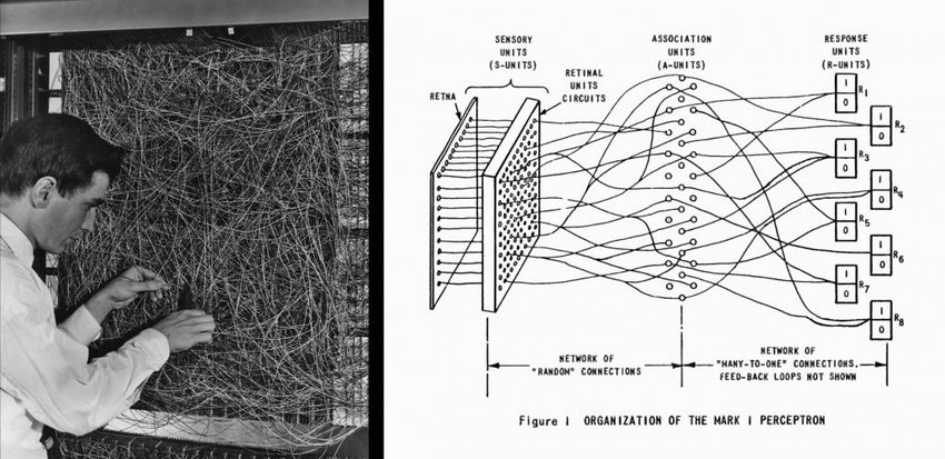
Figure 1: Rosenblatt’s 1957 Perceptron [2].

What about adding more layers? As we know, adding more layers to a neural network can significantly enhance its ability to extract higher-level information. However, when Fukushima wrote this paper, there was no algorithm to enable self-organization in multilayer neural networks (although this was later achieved by the backpropagation algorithm). Therefore, systems claiming self-organization did not fundamentally go beyond the three-layer perceptron framework.

To solve these problems and achieve unsupervised learning, the author proposed a new hypothesis to model synaptic strengthening.

Hypothesis

Before introducing the new hypothesis, let’s examine the issues with prior assumptions, which the author categorized into three types:

• Synapse starts in a modifiable state, but if postsynaptic neuron is activated without the activation of presynaptic neuron , becomes inactive and no longer modifiable.
• Synapse has a random initial component, and only when both presynaptic cell and postsynaptic cell are activated, does strengthen. This type of synapse is known as a Brindley synapse.
• The postsynaptic cell has another synaptic input , known as a Hebbian synapse, which is initially inactive and only strengthens when both presynaptic cell and the control signal are active (this model assumes as a “supervisor”).

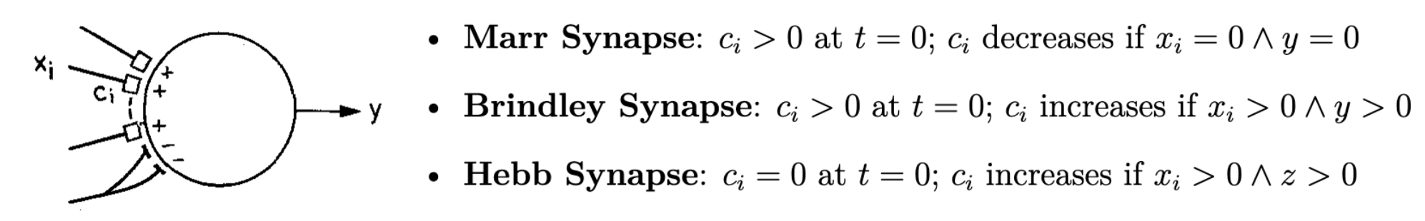
Figure 2: Mechanisms of three synapse types.

The first assumption is highly problematic: if a single incorrect signal occurs, the synapse could irreversibly change, potentially rendering the network functionally “extinct” over time. Brindley synapses offer partial self-organization, but the randomness of initial synapses may not ensure meaningful connection patterns, and large-scale networks have not proven Brindley synapse effectiveness. Hebbian synapses rely on an external supervisor signal , which is biologically unreasonable.

To address these issues, the author proposed a new hypothesis. For synapse strengthening between neurons and via synapse , two conditions are required:

1. Presynaptic neuron of synapse is activated.
2. None of the neurons near postsynaptic neuron respond more strongly than .

Condition two implies that synaptic strengthening is unique within its local neighborhood. This uniqueness allows each neuron in the network to develop a distinct response, enhancing the network’s feature differentiation ability. Moreover, if a neuron malfunctions, other neurons can take over its role, similar to self-repair functions in biological neural networks. This new hypothesis, akin to the brain’s mechanism of supplying nutrients only to the most responsive neurons, also has biological plausibility.

Next, let’s model the neurons and network structure.

Neuron Modeling

The neurons in the Cognitron use a “shunting inhibition” mechanism. In traditional linear inhibition, if an excitatory signal and an inhibitory signal are present, the final pulse strength is generally represented as . Shunting inhibition refines this response, preventing over-activation by using a division-based model. The final output behaves similarly to an activation function, producing non-negative values proportional to the pulse strength. Denote as inputs from excitatory synapses and as inputs from inhibitory synapses. Each neuron’s output is defined as:

where and are the conductance values for excitatory and inhibitory synapses, both non-negative. is defined as:

Let represent the sum of all excitatory effects and the sum of all inhibitory effects:

The neuron output formula can be simplified as:

In the Cognitron, synaptic conductance values and increase over the learning process (which is intuitive); as conductance increases and and , the above formula approximates:

At this point, the output depends on the ratio , not on their difference. Thus, even if conductance increases with learning, as long as excitatory synapses and inhibitory synapses increase proportionally, the neuron output converges to a stable value instead of diverging. We assume excitatory and inhibitory inputs increase proportionally, represented by:

where is the total signal strength. If , the neuron output can be transformed as:

We find that this input-output relationship is consistent with the Weber-Fechner law’s logarithmic relationship, expressed as an S-shaped response curve represented by the tanh function.

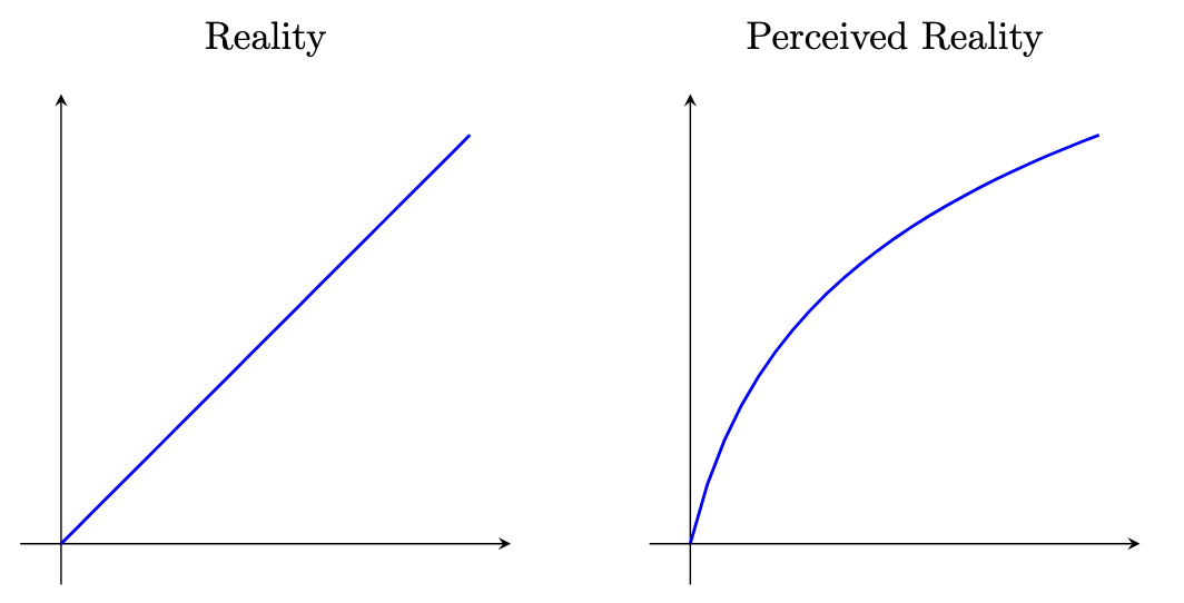
Figure 3: The Weber-Fechner Law – perceptual curve vs. physical reality.

This formula is often used as an empirical formula in neurophysiology to approximate the nonlinear input-output relationships in sensory organs and animal sensory systems. The author believes that since these types of neural elements closely resemble biological neurons, they should be well-suited to various visual and auditory processing systems.

Cognitron Structure

Based on the new hypothesis, let’s dive into the structure of Cognitron. Cognitron is composed of multiple neural layers with similar structures, arranged sequentially. The -th layer (labeled ) consists of excitatory neurons and inhibitory neurons , where represents the two-dimensional position of neurons.

The excitatory neuron receives pulses from excitatory neurons in layer and from inhibitory neurons . Here, represents the connection area for the neuron, and represents the coordinates of all excitatory neurons in . If we denote the synaptic conductance as and , the output of can be given by the following formula:

The inhibitory neuron receives weighted input from neighboring excitatory neurons and outputs to :

where represents the weight of the inhibitory synapse, with the sum of weights equal to 1:

Figure 4 shows the connections between and .

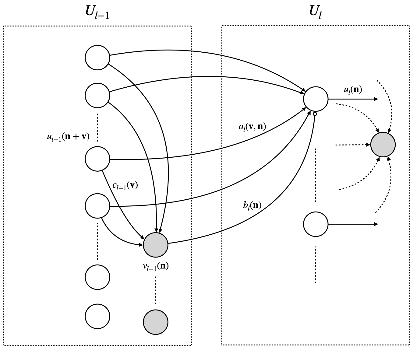
Figure 4: Visualization of Cognitron Structure.

It can be seen that the receptive field of neuron overlaps with the receptive fields of the excitatory synapses connected to . Now, let’s model the synaptic strengthening mechanism. Based on the hypothesis, let be a Boolean function indicating whether or not a synapse should be strengthened. If responds more strongly than any other neuron within neighborhood , it takes a value of 1:

When , the changes in and depend on whether or .

1. When
   
2. When
   
   and are positive constants, with . In the first case, if and no neurons in the neighborhood respond, the synaptic strengthening amount is relatively small. In the second case, when , since , the synaptic strengthening is more significant, with suppressed by the square of the input signal from the previous layer, thereby moderating the inhibitory synaptic strengthening amount, in line with the “winner-takes-all” rule in the hypothesis.

Quantitative Analysis of the Algorithm

The author conducted extensive analysis based on the Cognitron algorithm; here, we summarize some key insights without delving into the detailed analysis:

1. After learning, the number of neurons with strong responses significantly decreased, exhibiting sparsity, which helps the network distinguish between different input patterns.
2. When , excitatory synapses tend to strengthen more than inhibitory synapses; when , inhibitory synapses may strengthen more.
3. Repeated exposure to the same stimulus enhances the output connections between neurons . As gradually increases, the output approaches 1, indicating that the network has “learned” a specific output pattern.

In addition to the basic algorithm, the author modeled lateral inhibition phenomena, but for simplicity, this is not covered here. Lateral inhibition reduces the response of surrounding neurons when a neuron responds strongly to a specific stimulus, promoting sparse connections.

Layer Connections and Axonal Branching

Finally, let’s define how the network layers connect. This paper discusses three different methods for defining the receptive field of each layer. The first method maintains the same receptive field size at each layer, but to achieve sufficient receptive field coverage, more layers are required, complicating the network structure. The second method increases the receptive field size layer by layer, allowing for larger receptive fields with fewer layers, but the similarity of responses in the final layer (output layer) weakens the network’s ability to distinguish different stimuli.

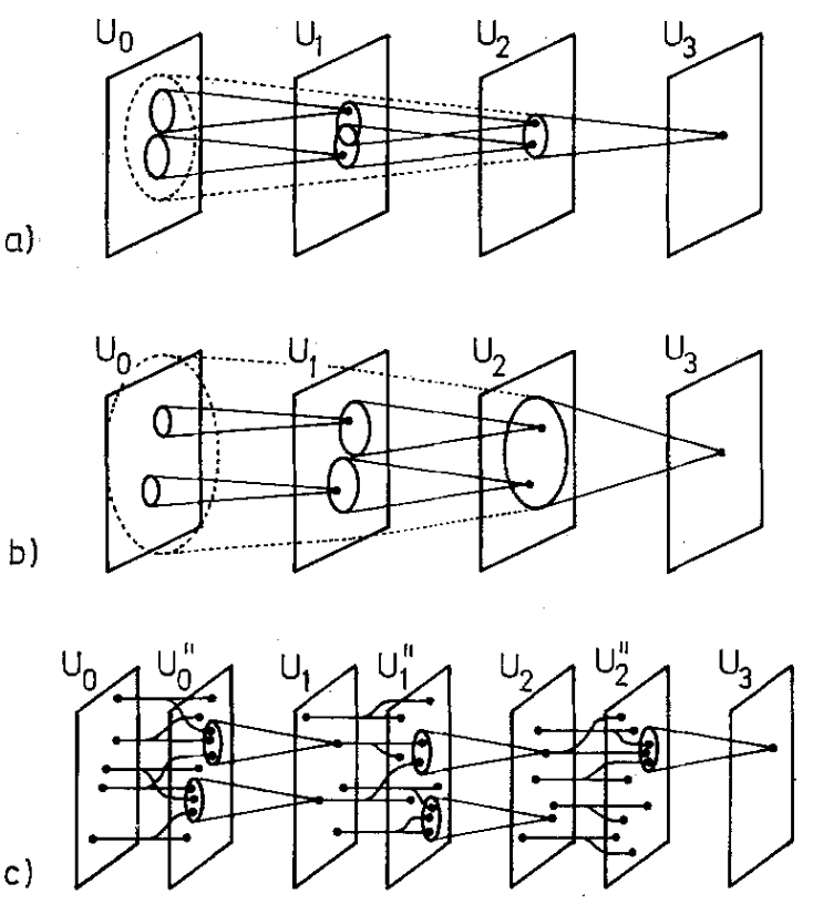
Figure 5: Three methods of defining layer connections.

The third method (5c), chosen in this paper, uses probabilistically distributed axonal branches as the layers deepen, extending the receptive field without excessive overlap.

Cognitron adopts the third method. Suppose each excitatory neuron has axonal branches, where one branch transmits directly forward, while other branches undergo probabilistic displacement. Let be the permutation operator for . We have:
$$
u^{\prime}l(\mathbf{n}, k) = P{lk} { u_l(\mathbf{n}) } \quad (k \neq 0)
$$
In computer simulations, this study focused on , where the axon divides into two branches, one direct and the other probabilistic.

The output of axonal branched neurons is redefined as:
$$
u^{\prime}l(\mathbf{n}) = \varphi \left[ \frac{1 + \sum{k=0}^{K} \sum_{v \in S_l} a(\mathbf{v, n}, k) \cdot u^{\prime}{l-1}(\mathbf{n+v}, k)}{1 + b_l(\mathbf{n}) \cdot v{l-1}(\mathbf{n})} - 1 \right]

\begin{align*}
u_{l-1}(\mathbf{n+v}) &\rightarrow u^{\prime}{l-1}(\mathbf{n+v}, k) \
a(\mathbf{v, n}) &\rightarrow a(\mathbf{v, n}, k) \
c{l-1}(\mathbf{v}) &\rightarrow c_{l-1}(\mathbf{v}, k) \
\sum_{\mathbf{v} \in S_l} &\rightarrow \sum_{\mathbf{v} \in S_l} \sum_{k=0}^{K}
\end{align*}
$$

Computer Simulation and Conclusion

In the simulation, the author used four network layers, each with excitatory neurons and the same number of inhibitory neurons. The connection area , neighborhood area , and range of lateral inhibition were all carefully set. The network was exposed to 12x12 images of numbers 0 through 4, with responses recorded at each layer.

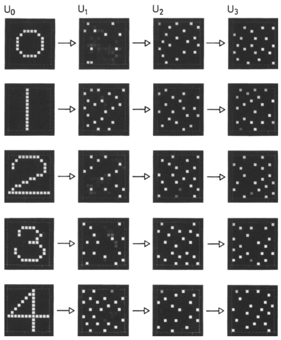
Figure 6: Response patterns for numbers 0-4.

The study found that after multiple exposures, Cognitron could achieve self-organization, with most cells in the deepest layer () selectively responding to specific stimulus patterns.

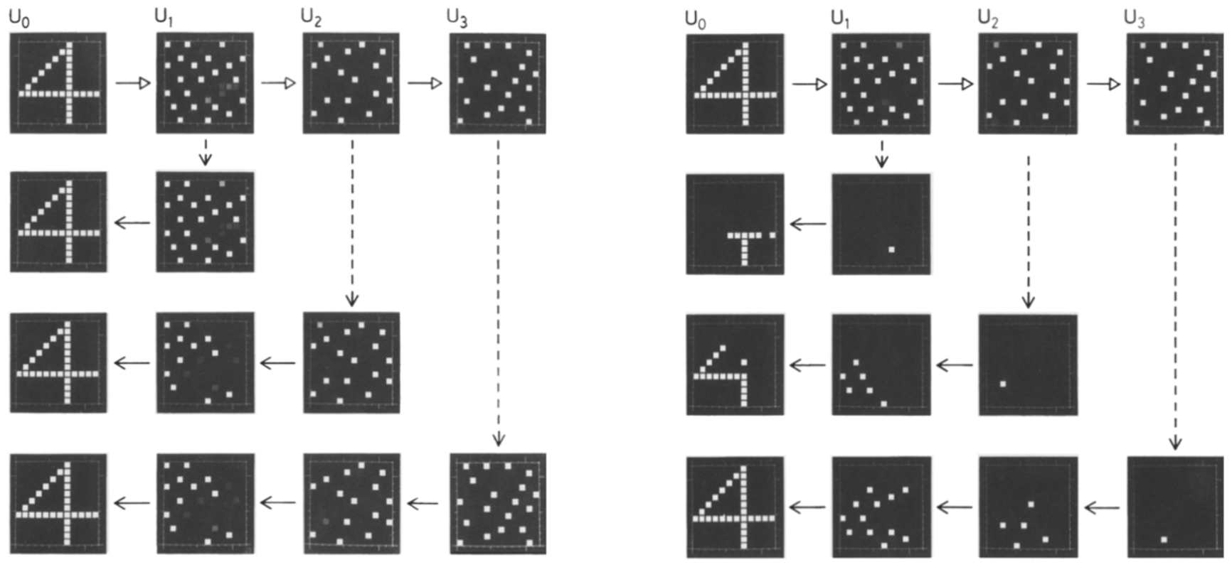
Figure 7: (Left) Reverse reconstruction from the normal responses of a single layer of cells. The first row shows the normal response to the stimulus “4,” recorded during the 20th cycle of pattern presentation. The second, third, and fourth rows respectively show the results of reverse reconstruction from the normal response patterns in layers U1, U2, and U3. (Right) Reverse reconstruction from the normal response of a single cell. The first row shows the normal response to the stimulus “4.” The second, third, and fourth rows respectively show the reverse reconstruction results from the strongest responses of individual cells in layers U1, U2, and U3.

To verify the effect of synapse organization, researchers conducted a reverse reconstruction experiment, where the flow of information through synapses was assumed to be reversed, allowing them to observe the responses of each layer’s cells. Results showed that using this method, it was possible not only to deduce specific numbers from the responses of 144 neurons but also to backtrace input patterns from single cells in deeper layers to earlier layers, demonstrating that each neuron’s response was unique. This indicates that Cognitron developed a self-organizing ability specific to this task. (Results shown in Figure 7)

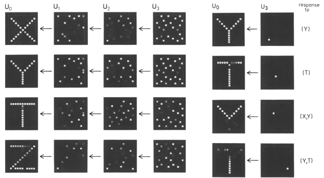
Figure 8: Cognitron’s network layer and single neuron reverse inference capabilities when receiving similar stimulus patterns.

In the final set of experiments, as shown in Figure 8, the author explored Cognitron’s ability to respond to similar stimulus patterns (e.g., “X,” “Y,” “T,” and “Z”) using the same testing method as described above. Results showed that even though these letters shared common components (e.g., the head of X and Y, or the tail of Y and T), Cognitron was still able to distinguish between and respond differently to them, indicating its capacity to differentiate similar information.

A Short Summary

To summarize, by following a new synaptic organization hypothesis (“winner takes all, loser gets none!” albeit with a hint of humor), Cognitron successfully achieved self-organized learning, with many aspects of its algorithm displaying similarities to the biological brain. Due to its multi-layered structure, Cognitron could handle complex tasks in information processing more effectively than traditional brain models or previous artificial neural networks. However, research also pointed out that Cognitron lacks a complete capability for pattern recognition. For example, to fully enable Cognitron to perform pattern recognition tasks, additional functions such as spatial pattern normalization or completion would be needed—somewhat akin to our aim to achieve AGI. Yet, as we see even in 2024, the road ahead remains challenging.

Following Cognitron, Kunihiko Fukushima authored another paper introducing “Neocognitron,” an upgraded version of Cognitron designed to make neural network recognition invariant to factors such as image rotation. Feel free to read it if you’re interested!

Conclusion

The “Tracing Back” series is now drawing to a close. In the next issue, we’ll cover the foundational language model paper A Neural Probabilistic Language Model, followed by a final issue with code reproductions of key papers. While writing these articles, I noticed an interesting trend: the earlier the work, the more it emphasized the connection between the “biological brain” and the “artificial brain.” In the Cognitron paper, we can see traces of neuroscientific influence throughout, which the researchers leveraged. The previous article on backpropagation, while closer to modern AI, already showed fewer of these connections. Nevertheless, even in that paper, the authors mentioned that since the biological brain does not follow backpropagation, we should look for more “natural” learning algorithms.

Today, most AI research is categorized as a purely computational field, aiming for novel engineering ideas and constantly pushing SOTA in various projects. However, there’s a notable lack of research focused on understanding “why it works.” This shift sometimes raises questions about our goals: has the purpose of our research diverged from the past? Are we still on the path to achieving AGI? We’ll leave a question mark here and let time reveal the answer.

Lastly, creating these articles has not been easy, so if you’ve read this far, please give it a like! (＾3＾)

References

[1] Fukushima, K. (1975). Cognitron: A self-organizing multilayered neural network. Biological Cybernetics, 20(3–4), 121–136. https://doi.org/10.1007/bf00342633

[2] Singh, K., Ahuja, A., Chatterjee, T., Pritam, S., Varma, N., Jain, R., Sachdeva, M. S., Bansal, D., Trehan, A., Hajra, S., Kar, R., Basu, D., Peepa, K., Anil, I., Banashree, R., Apabi, H., Ghosh, S., Samanta, S., Chattopadhay, A., & Bhattacharyya, M. (2019). 60th Annual Conference of Indian Society of Hematology & Blood Transfusion (ISHBT) October 2019. Indian Journal of Hematology and Blood Transfusion, 35(S1), 1–151