Tracing Back to the Origins | A Neural Probabilistic Language Model
Introduction
A Neural Probabilistic Language Model, first published in 2000, used neural networks to address language modeling for the first time. Although it didn’t receive much attention at the time, it laid a solid foundation for the application of deep learning in solving language modeling and many other NLP problems. Later researchers stood on the shoulders of Yoshua Bengio, achieving more breakthroughs, such as Tomas Mikolov, the creator of Word2Vec, who proposed RNNLM and then Word2Vec based on NNLM. The paper also introduced an early idea of representing words as low-dimensional vectors rather than one-hot encoding. Word embeddings, as a byproduct of language models, have played a critical role in subsequent research, offering researchers a broader perspective.
Model
The goal of statistical language modeling is to learn the joint probability function of word sequences. The author addresses the dimensionality explosion problem (due to the vast number of words) by learning distributed representations of language. A statistical language model can express the conditional probability of the next word given all previous words, as shown below:
- (w_{t}) represents the (t)-th word
- (w_j^i= = (x_{i},x_{i+1},…,x_{j}))
In fact, the word at a given position in a word sequence is more dependent on nearby words. Consider the n-gram model (which performs best when (n = 3)); the conditional probability of the next word can be expressed using only the previous (n-1) words:
However, this approach has limitations. On one hand, words beyond the two nearest words may also contain implicit semantic information. On the other hand, this method does not account for word similarities. (For example, seeing the sentence “the cat is walking in the bedroom” in the training corpus should help generalize the sentence “A dog was running in a room” since “dog” and “cat,” “The” and “A,” and “room” and “bedroom” share similar semantic and syntactic roles).
The following derivations are expressed using matrix operations, so let’s clarify some notations used in this paper:
- (v) is a column vector; its transpose is (v’)
- (A_{j}) represents the (j)-th row of matrix (A)
- (x.y= x’y)
Fighting the Curse of Dimensionality with Distributed Representations
In summary, the proposed method can be summarized as follows:
- Find the distributed feature vector for each word in the vocabulary. (A real-valued vector of dimension (m))
- Represent the feature vectors of words in the sequence as a joint probability function of the word sequence.
- Simultaneously learn the word feature vectors and the parameters of the probability function.
The Neural Model
Variable Notations and Overall Process
- Vocabulary (V)
- The training set is a sequence of words (w_{1},w_{2},…,w_{T}), each word from the vocabulary (at this stage represented in its original form).
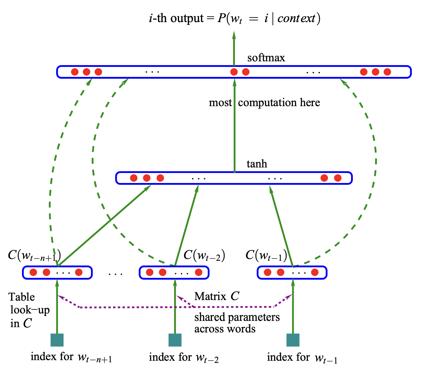
- Our objective is to find a model function (f(w_{t},w_{t-1},…,w_{t-n+1}) = P(w_{t}|w_{1}^{t-1})).
We can decompose the model function (f(w_{t},w_{t-1},…,w_{t-n+1}) = P(w_{t}|w_{1}^{t-1})) into two parts:
- Find a mapping set (C), where for any word (i) in the vocabulary (V), we can find the corresponding feature vector of the word through (C(i)). The size of (C) is (|V|\times m), and all elements are trainable parameters.
- Based on the words, express the probability function (f(i,w_{t-1},…,w_{t-n+1})=g(i,C(w_{t-1},…,C(w_{t-n+1})))
In general, the (f) function is a composition of two mappings, (C) and (g). (C) is a parameter shared among all words in the text. Thus, the parameters to determine are (\theta = (C,w)), where (w) represents the parameters of the probability function. Training is done by maximizing the log-likelihood loss function over the training set, as expressed below:
where (R(\theta)) is a regularization term.
Description of Computation Process
Forward Computation
(a) Compute forward for the word features layer:
where (x(k)) represents the feature vector of the word (k) positions away, and is an (m)-dimensional vector.
(b) Compute forward for the hidden layer:
where:
- The number of hidden layer neurons is (h).
- (x) is a vector of size ((n-1)m) (parameter).
- (H) is a matrix of size (h\times (n-1)m), outputting a vector of size (h) (total output of hidden layer, each node outputs a number) (parameter).
- (d) is a vector of size (h) (parameter).
- (a) is a vector of size (h).
(c) Compute forward for output units in the (i)-th block:
- (s_i\leftarrow 0)
- Loop over (j) in the (i)-th block
- (y_j\leftarrow b_j +a.U_j)
- If (direct connections) (y_j\leftarrow y_j+x.W_j)
- (p_j\leftarrow e^{y_j})
- (s_i\leftarrow s_i+p_j)
Computation in Output Layer
Indexes indicate the word position in vocabulary (V). Each (y_{i}) is a forward-computed probability value. Since softmax normalization is applied at the end, the exponent (p_{i}) is computed.
- (U_{j}) is a vector of size (h) (one for each word in (|V|)) (parameter).
- (W_{j}) is a vector of size (m) (whether direct connections exist can be determined by training; if all are zero, there are no direct connections) (parameter).
The result is the probability for each word, which is then used to update the log-likelihood function. This can be computed using sentences from the training set, where each sentence is a word sequence, allowing calculation of the log-likelihood function:
Using Deep Learning Tools
With modern deep learning tools, these problems can be solved quickly. Essentially, this involves a feedforward process with one hidden layer (using (\tanh) as the activation function) and an output layer, with a direct connection from the original input (x) to the output layer. Note, however, that the input layer is also trainable.
- (x) is a vector of size ((n−1)m) (parameter).
- The middle (hidden) layer has (h) neurons with (\tanh) as the activation function.
- The output layer has (|V|) neurons.
Summary
This paper introduces neural networks into language model construction, similar to the development of neural networks in other fields. The core idea is to use neural networks to learn feature representations of the input and to combine these representations to accomplish related tasks. Word embeddings, or distributed word representations, are conceptually similar to convolution in images; the fundamental unit in language is a word, while in images, it is various visual features. The key to deep learning is to learn these features and utilize them. Neural networks essentially transform the feature space, and one might consider that human understanding of natural language results from relatedness in a mental language space, while neural networks can simulate the brain to find such relationships.